
Christmas comes in June for energy geeks and graph junkies. Every year, the Energy Information Administration of the Department of Energy releases its Annual Energy Outlook (AEO), a compendium of 30-tear forecasts and analyses of energy sources and uses. The 212 page .pdf file contains tables, bar charts and area graphs galore, enough to provide blog fodder at least until Christmas (the December one).
This week’s installment is a look at production decline curves from selected shale gas plays. The extreme rates of decline experienced in these wells has interesting and far-reaching policy implications, although this angle is rarely described in the mainstream press. For the energy operator, the performance of his wells in aggregate determine the success or failure of his enterprise. For the nation, shale well performance has become a key factor in energy policy and planning.
Reserves and price projections are the key to everything. I promise to keep this understandable at a general business level.
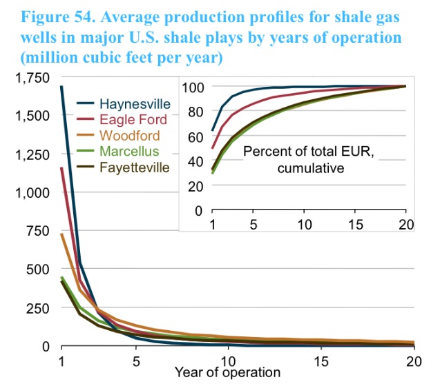
The curves in Figure 54 at left represent averages for five different shale plays; each well is an individual. But what this curve fails to make explicit is the fact that there are very few wells in these shale gas plays with more than four years of history; the rest is projection.
Engineers commonly use decline curves (pdf) as a primary tool for analyzing historical performance of producing wells and forecasting their future performance. The total accumulated past and future production of a well is termed its Estimated (or Economic) Ultimate Recovery (EUR). The EUR of gas wells is measured in billions of cubic feet (BCF). The estimate of future production is termed “remaining reserves”.
Since a resource company’s primary asset is its reserves, these squiggly lines have a lot to do with a company’s financial performance. Truth be told, decline curve analysis can be subjective instead of scientific, particularly early on in a well’s life. Tight rocks like shales typically exhibit this characteristic “hyperbolic” shape, declining precipitously in the early years; EUR depends on how quickly the rate “breaks over” to a lower, more sustainable rate.
 EIA’s Table 17 (click any image to enlarge) shows how reserve estimates have changed in the last three AEOs. In particular, the estimate for average recovery of a well in Louisiana’s Haynesville Shale was 4.59 billion cubic feet (BCF) per well in AEO2010, 3.58 BCF in AEO2011, and only 2.67 BCF per well in this most recent AEO2012. Just as surprising is the inset graph in Figure 54 above, which suggests that a typical Haynesville well produces >95% of its reserves in the first 5 years. The wells produce at phenomenal rates to begin with, but decline rapidly due to the constrained flow properties of ultra-tight shale rocks.
I don’t have any insight on the EIA’s methodology or statistics, but it would appear that as data accumulates with time, the Haynesville per-well reserves have decreased. Back in 2008, Chesapeake Energy made a big splash as the Haynesville pioneer; their estimate at the time was that Haynesville wells would average 6.5 BCF each. (At the time, gas prices were north of $8.00 per mcf at the wellhead.)

All that “flush gas” coming on the market created a temporary glut and drove natural gas prices into the basement. As recently as 2004, energy in the form of gas cost more than the equivalent amount of energy as oil (see Figure 34, left). The horizontal drilling and fracking concepts were first proved in the Barnett Shale of Texas; the phenomenal early success in the Haynesville in turn ignited shale plays in across the country, and now those ideas are spreading internationally, too.
How big a difference does all this make? For an energy company, it is all about reserves x price; when one or both goes south, it is bad news. When you produce disappointing reserves into declining price, it can be disastrous.
 The table at right is a grossly simplified look at the economics of developing the EIA’s typical well from the 2011 and 2012 studies. Gross revenue is reserves times price; in this example the gross revenue for a 3.58 BCF well, given $4.50/mcf gas prices (early 2011 prices) over the well’s life would generate $16.1 million in gross revenue (far right column). After deducting landowner royalties, state severance taxes and lease operating expenses, the owner’s net is almost $10.8 million, enough to repay the assumed $7.5 million cost to drill and equip the well and leave a $3.3 million profit. (This analysis ignores overhead, income taxes and the time value of money. It also ignores the up-front cost of the lease, the rights that allow the driller to drill, which can be very significant.)
But if the well’s performance disappoints and the reserves turn out to be 2.7 BCF (per AEO2012) instead of 3.6 BCF, drilling becomes a breakeven proposition, even if the price hangs in at $4.50. With the price falling to $2.50, it’s a disaster. The operator takes home only 50¢ on $1.00 of his initial drilling investment. That’s called “destroying value”, and it doesn’t matter if you’re an oil man, a shoe salesman or a chicken farmer, you understand that that’s bad for business. (Politicians may not get it, and there’s not a lot we can do about that.)
Operators have mostly responded rationally to the current oil/gas price situation. The Haynesville produces “dry gas”, i.e. without associated liquid hydrocarbons. A modest amount of oil or condensate produced along with the gas can radically alter drilling economics. Consequently, most operators have refocused their attention away from the Haynesville and other dry gas plays to gas/condensate plays like the Eagle Ford of south Texas or to pure oil plays like the Bakken of North Dakota. In the Eagle Ford, the gas price matters little because the economics are totally driven by the condensate.
Historically, 60-70% 0f domestic rigs targeted gas. Now, only 25% of the rig fleet drills for gas.
Long term trends? I look for the historically wide price spread of gas vs oil to close somewhat. Few operators will be able to deliver gas to the market profitably under the current price regime. We have already seen the total production curve for the Haynesville peak and begin to decline.
Is this the end of the “shale bubble”? Hardly. The shales are everywhere. Each one has different characteristics and a different breakeven price.
I suspect that price stability in the $4-$5 range would support an active gas drilling industry. Even at that level, gas would still provide a huge price advantage compared to gasoline as a transportation fuel.
Natural gas is clean, abundant and American; it makes up nearly 25% of our nation’s total energy consumption. Of the fuels in our energy mix, gas is the most versatile, useful for electrical generation or for transportation. Domestic drilling is a true, private sector “shovel ready” jobs program that could be kicked into high gear overnight without tax credits and DoE loan guarantees.
Cross-posted at Maley’s Energy Blog.
Follow @VladimirRS
!function(d,s,id){var js,fjs=d.getElementsByTagName(s)[0];if(!d.getElementById(id)){js=d.createElement(s);js.id=id;js.src=”//platform.twitter.com/widgets.js”;fjs.parentNode.insertBefore(js,fjs);}}(document,”script”,”twitter-wjs”);


Join the conversation as a VIP Member